6. Atmospheric particles

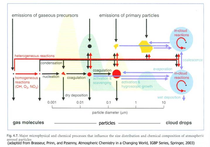
As we discussed in Chapter 2, atmospheric aerosols can be either emitted directly or produced by gas-to-particle conversion. On a global scale, both direct emissions and gas-to-particle conversion are important. The figure below shows the main processes that influence atmospheric aerosols.

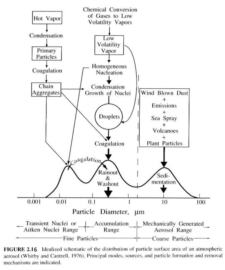
The resulting size distributions from these processes was given in a figure in Chapter 2, which is repeated below.

Two features of aerosol are partcularly important for understanding the roles that aerosols play in atmosphere’s chemistry and radiative balance. There are the size distributions and the chemical composition. If we know these two properties very well, then by doing some laboratory work, we can descibe the aerosol’s chemical, microphysical, and optical properties. Our goal in this chapter is to describe the physical and chemical processes that create the aerosol distributions that are observed.

Aerosol sources.

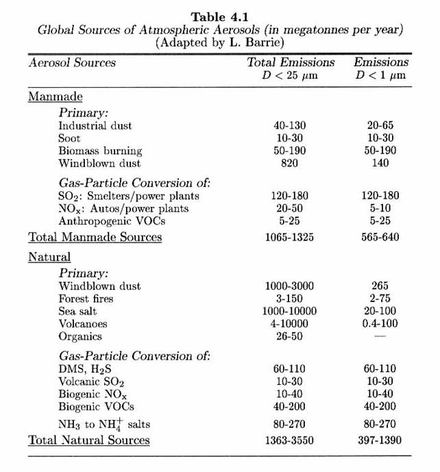
The following table presents the sources of tropospheric aerosols.

1. Anthropogenic are slightly less than natural.
2. More than half the sulfur is anthropogenic.
3. Biogenic VOCs are globally more important than anthropogenic VOCs

This table gives the global estimates, but the distributions are highly variable. Urban areas have about 10 times the number of particles as rural areas, which generally have larger aerosol concentrations than remote areas.

We have two types of mixtures.

1. Externally mixed. Aerosol particles having different chemical compositions are in the same airmass.
2. Internally mixed. Each individual aerosol particle contains a mixture of chemicals.

Size distributions.

Aerosol sizes vary over several orders of magnitude, from a few nm to 10 of microns. Aerosol number concentrations (number/volume) also vary over orders of magnitude, from a few all the way up to 10⁷ to 10⁸ cm^-3. It should be of no surprise that urban areas generally have much higher aerosols concentrations than rural or remote areas.

We are interested in the size distributions of these aerosols, just as we are interested in the chemical composition as a function of aerosol size.

Let’s go back to the figure that I showed before to get a rough idea about size distributions.

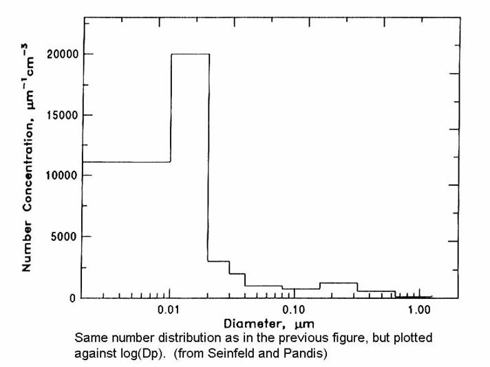
1. fine particles (diameters < 2 mm). These generally come from gas-to-particle conversion. They consist of the nucleation mode (diameters < 0.1 mm) and the accumulation mode (0.1 < diameters < 2mm).

2. course particles (diameters > 2 mm). These generally come from mechanical processes, such as the sea spray, windblown dust, particles from tires and breaks, etc.)

Some definitions. Both diameter and radius are used to specify aerosol size. Seinfeld and Pandis use diameter, D_p. We will occasionally use radius, R_p.

Aerosols are often measured with instruments that segregate the aerosols by size, since the size of the aerosol is an important quantity to know in order to understand the processes that produced the aerosols and their likely effects on humans.

For any size bin labeled i:

1. N_i = the number of aerosol particles per cm^-3 of air in that size bin (units = cm^-3).

2. n_i = is the number of aerosol particles per cm^-3 of air per unit size interval. (units = mm^-1 cm^-3).

3. Thus, in any given size interval, N_i = n_i DD_pi, where DD_pi is the size of the interval.

4. The total number of particles comes from adding together all of the particles in the different size bins:

N = S_i N_i = S_I n_i DD_pi

If the size bins could be made infinitely small, then we can use an integral:

n_N(D_p) d D_p = the number of particles per cm^‑3 of air having diameters in the range D_p to D_p + DD_p.

N = ò₀^∞ n_N(D_p) d D_p

or

n_N (D_p) = dN / dD_p.

This is a useful concept for a few reasons.

1. It allows us to get a good idea of the actual distribution even when particle measuring instruments do not have equal sized bins.

2. We can integrate the curves directly to get the total number of particles. This second point is particularly important when we want to get a quick idea of the total number, surface area, or volume of the observed aerosols.

We can take this concept of size distribution function to determine the surface area, volume, and total mass of the particles. Generally, we assume that the particles are spherical. We are really considering the densities of surface area, volume, and total mass, i.e. the amount of each quantity per unit volume of air.

We get the following expressions:

Surface area. The surface area is important for heterogeneous reactions.

The surface area per unit diameter is given as:

The total surface area density can be found by integrating n_s:

Volume. The volume determines the total amount of a chemical is in the aerosol.

The volume per unit diameter is given as:

The total volume density can be found by integrating n_V:

Mass (assuming a uniform density).

where the units for r are g cm^-3.

Thus,

Actually, aerosol masses are usually reported as mg m^-3. The typical mass concentrations range from less than 1 mg m^-3 in clean environments to 10’s to perhaps even a few hundred mg m^-3 in more polluted environments.

Because the size distributions span such size ranges, it is often best to look not at the size distributions as a function of the diameter, but instead, to think of them as a function of the logarithm of the diameter. Thus, we get the following functions for the number, surface area, and volume distributions:

Let n_N(log(D_p)) d log(Dp) be the number of particles per cm^-3 of air with diameters in the range of log(D_p) to log(Dp) + d log(D_p).

Then we can define the following relationships:

To get the total number, we simply do the integratls:

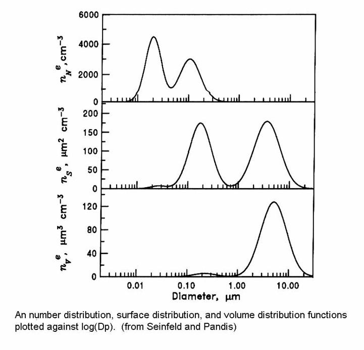
The distributions of number, surface, and volume are shown in the figure below. Note that the greatest number of aerosol particles is in the smallest range, the surface area is mostly in the intermediate range, and the volume is greatest in the large particle range.

We are often most interested in the mean particle diameter and the size variance:

Log-normal distribution. The most frequently used analytical expression that is used to attempt to fit observed particle size distributions is the sum of several log-normal distributions:

where “i’ represents a single log normal distribution. In each log normal distribution, three parameters must be specified: N_i, the total aerosol number concentration, D_pi, the diameter at the value of the peak number concentration, and s_i, the geometric standard deviation of the distribution. 67% of the particles have diameters between D_pi / s₁ and D_pi x s_i.

Often, two or three log-normal modes are used to fit the observed distributions. Note that 3 parameters are required to fit each log-normal distribution that is used.

One nice feature of the log normal distribution is that the surface area and volume distributions are also log normal with the same s_i.

Atmospheric fates of aerosol particles.

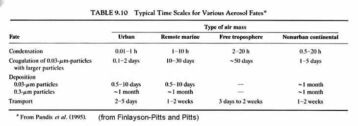
There is a great deal of physics and microphysics involved with the removal of aerosol from the atmosphere. We would need to discuss aerosol aerodynamics, fall speeds, Brownian motion, and coagulation. Instead, we will simply mention the time scales for removal of aerosols by different mechanisms and for different size ranges of aersol diameters.

While particles larger than 2 mm are effectively removed by gravitational settling, and particles with diameters < 0.1 mm are able to diffuse through the air, and thus end up on surfaces, particles with diameters in the range of 0.1 to 2 mm are not effectively removed by either mechanism. They thus tend to accumulate in the atmosphere.

The fates of aerosols are given in the following table.

Atmospheric sources of aerosol particles: Gas-to-particle conversion.

Gases can condense on existing aerosols, called heterogeneous nucleation, or can condense molecule by molecule to form an aerosol, called homogeneous nucleation. If the condensing molecule is water, homogeneous nucleation almost never occurs. Almost all water vapor condenses on pre-existing aerosols of some other chemical composition. This situation is not true for important chemical species like sulfuric acid or organic acids, which can form aerosols by homogeneous and heterogeneous nucleation. We will look now at these two processes.

Homogenous nucleation.

Up to now, all of our discussions about multiphase systems have assumed that the interface surface is flat. For a molecular point-of-view, this would be true for drops as large as 10 mm or more. However, for small drops, say on the scale of 10 nm, the curvature of the drop is quite large.

Consider the formation of a drop from some substance. As the molecules come together, they form electrostatic bonds and a release of energy. At the same time, they are forming a surface and work is required to expand the surface in the presence of intermolecular forces that are trying to minimize the surface. As the molecules are coming together, the work required to form the surface is greater than the energy generated by condensation. It is not until enough molecules have come together, that the energy gained from condensation is greater than the work required to build the surface. The critical radius for which the change in free energy is maximum is given by the equation:

R_p^* = 2s V_l / kT ln S

where s is the surface tension, V_l is the volume occupied by a molecule in the liquid phase and S = p_A / p_A^o, is the saturation ratio. p_A is the vapor pressure over the curved surface and p_A^o is the vapor pressure over a flat surface.

This is an equilibrium condition, although the equilibrium is metastable because we assume that the equilibrium assumption holds even though the particle may be growing or shrinking. Rearranging this expression:

which can be rewritten in other terms as:

where M = molecular mass; ρ_l = mass density of the liquid; and R = 8.314 J mole^-1 K^-1 . V_l is the volume of the drop = 4/3 p R_p³

Since R_p is in the denominator of the exponential, we can expect that the smaller the particle radius, the greater the vapor pressure. Thus small particles have high equilibrium vapor pressures and tend to evaporate.

The physical explanation for this effect is that the smaller the radius, the greater the exposure of any molecule on the interface with the gas phase. Since each molecule on the interface has less contact with neighboring molecules, and thus less bonding, it is easier for each molecule at the interface to escape than it would be from a flat surface.

Why do we care if this effect – the Kelvin Effect – affects only very small particles? Where do particles come from? If they originate from gas-to-particle conversion, they start from individual molecules which are quite small, less than 1 nm or so. Tow molecules collide and stick together by electrostatic bonding to form a dimer. A third collides and sticks to form a trimer, and so on. However, at these early stages, the radius of the aerosol is very small and the equilibrium vapor pressure is very high. Evaporation to achieve the equilibirum condition predicted by the Kelvin Theory is fast. It is a constant battle between the nucleation of the aerosol and the evaporation of the aerosol.

For water, M = 0.018 kg/mole, r_l = 1000 kg m^-3, and s = 72 x 10^-3 Nt m^-1, R = 8.314 J mole^-1 K^-1. Assume T = 298 K.

Thus,

p_H2O ≡ e = e_s exp(2.1x10^-3/D_p)

where e_s is the equlibrium partial pressure of water vapor for a flat surface of pure water and D_p has units of mm.

The saturation ratio is defined as S = e/e_s. We can rewrite the above expression in terms of the saturation ratio:

S = exp(2.1x10^-3 / D_p)

The supersaturation, s, is defined as s = S-1 = exp(2.1x10^-3 / D_p) – 1.

The following figure shows the supersaturation as a function of aerosol diameter:

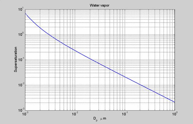
The formation of an aerosol or cloud drop begins at the molecular size near 0.001 mm. We see that the supersaturation that is required for nucleation to occur is quite large – greater than 5. This degree of supersaturation is essentially never reached in the atmosphere due to the presence of pre-existing aerosols. Thus, for pure water vapor, homogeneous nucleation has a very low probability of occurring in the atmosphere, except at low temperatures. I should state that just because the required supersaturation is large, it is not impossible for particles to form. It’s just very unlikely.

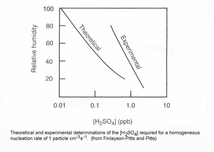
What about vapors other than water vapor? The vapor pressure over pure sulfuric acid at 296 K is 1.3 x 10^-8 atm. However, there is usually some water vapor in the atmosphere where sulfate exists. In the case of homogeneous nucleation of H₂SO₄, H₂O is also involved. This is called heteromolecular, homogeneous nucleation. The required concentration of H₂SO₄ and relative humidity is given in the figure from Finlayson-Pitts and Pitts. In the atmosphere, H₂SO₄ is typically less than 0.001 pptv because it is so readily deposited on surfaces and pre-existing aerosols.

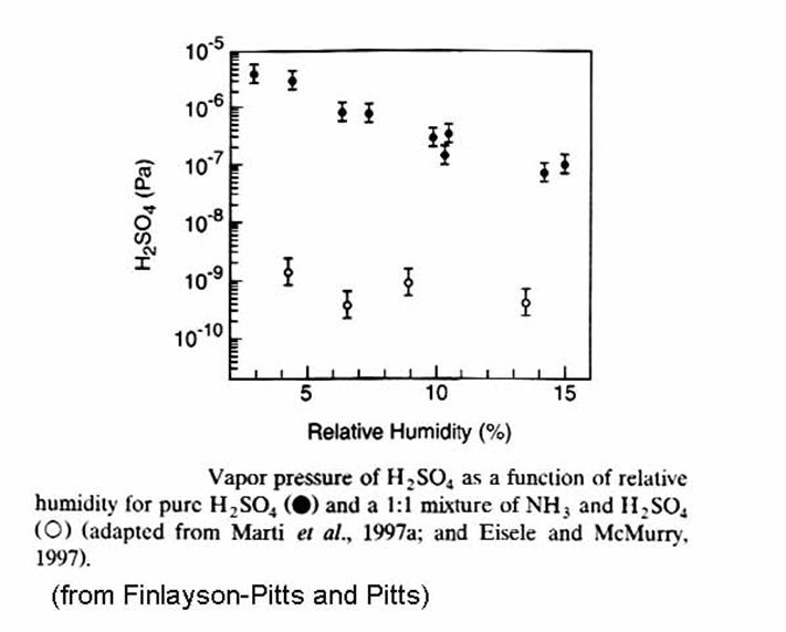
It should be noted that in clean regions of the atmosphere, sulfuric acid aerosols nucleate at a rate that is much greater than is predicted by binary nucleation theory. It has been proposed that the atmosphere contains a little ammonia, which greatly lowers the vapor pressure of H₂SO₄ above the aerosol, thus contributing to more rapid aerosol nucleation and growth, as can be seen in the following figure.

Seinfeld and Pandis discuss in some detail the thermodynamics of other common systems that include H₂O, H₂SO₄, NH₃, and HNO₃. NH₃ acts to neutralize the acidity of the aerosol, while HNO₃ and H₂SO₄ compete with each other (for low ammonia, sulfate tends to drive HNO₃ into the gas phase. Remember that H_HNO3^* = H_HNO3K_n1 / [H+].)

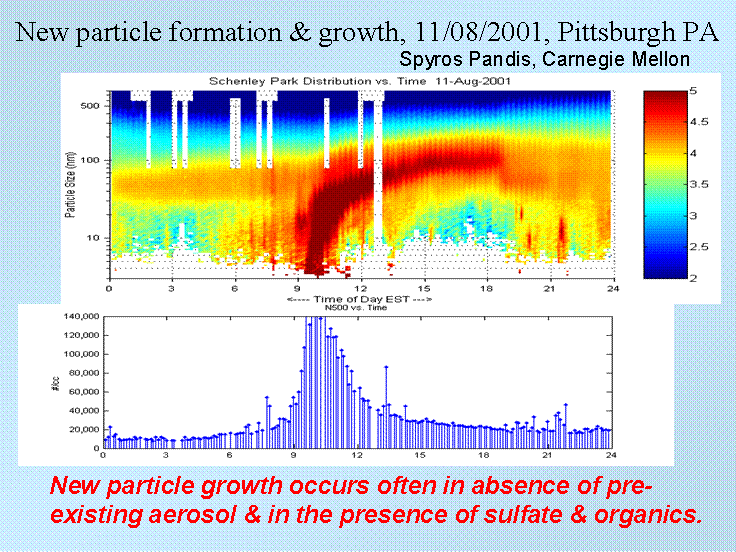
The recent, improved ability to measure particles in the nucleation mode has led to a number of interesting observations of homogeneous nucleation in the atmosphere. Some of the most interesting are homogeneous nucleation in urban areas, like Pittsburgh, which can be seen in the figure below. A front with rain had just passed through Pittsburgh, cleaning the air of pre-existing aerosol. However, the air contained both SO₂ and VOCs. Note that at just past 9, a large number of small nucleation particles emerge and then grow by collision coelescence and then vapor deposition into particles that are in the accumulation mode. As the particles coelece, the number per cubic cm of air drops. We would expect that the volume would grow, however.

Heterogeneous nucleation.

In this case, vapor condenses onto an existing particle.

In the presence of water vapor, we can get drops that consist mainly of water vapor.

The vapor pressure of water over the drop of radius R_p is determined by two factors:

1. the Kelvin effect, which raises the vapor pressure.

p_A = p_A^o exp{(2sM)/(RTr_lR_p)}

2. the Raoult effect, which lowers the vapor pressure for water vapor by occupying places at the air-liquid interface.

p_A = p_A⁰ (1 – χ_solute)

where

χ_solute = ([A(aq)])/([H₂O] + [A(aq)])

We can combine these two effects, make some approximations, and arrive at an expression for the vapor pressure over a drop that contains some foreign material:

where a_w is the water activity as was defined in Chapter 3, r_l is the density of the solution (which can often but not always be assumed to be the density of water, and M is the mass of the solution. We have assumed that all the sulfur has reacted and is in the form of sulfate, SO₄^2-.

The theory that incorporates the Kelvin and Raoult Effects is called Koehler Theory. Koehler theory is widely used in cloud microphysics to understand processes that are occurring in the atmosphere, such as cloud drop nucleation on cloud condensation nuclei (CCN).

The resulting curve has the form:

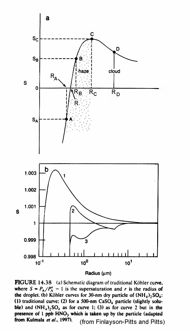
The behavior of the growing particle can be broken down into two regimes, which meet at the radius r_c, the radius that can be derived from Koehler Theory for the maximum saturation ratio.

Look at conditions in which S_K is less than S_C. Assume that we start with the particle in equilibrium (deposition = evaporation), so that S_K = S_amb, the ambient saturation ratio.

For R < R_C,

If a few molecules are added, then S_K becomes greater than S_amb and the particle then shrinks to come back into equilibrium.

If a few molecules are evaporated, then S_K becomes less than S_amb and the particle then grows to come back into equilibrium.

The haze then has a fairly narrow size distribution that is determined by the ambient saturation ratio, S_amb.

For R > R_C,

If a few molecules are added, then S_K becomes less than S_amb and the particle grows.

If a few molecules are evaporate, the S_K becomes more that S_amb and the particle shirnks all the way back to less than R_c to the size appropriate for the ambient saturation ratio.

The particle either grows to a much larger size, or it shrinks back to haze.

If S_amb > S_C, then the particle will grow for all circumstances.

Low volatility gases can be scavenged by existing aerosol, as well as water. Many of the chemicals can be low vapor pressure organic compounds that are formed in the oxidation process of other organic compounds. These absorbed organic compounds can influence the physical and chemical characteristics of the aerosol, including their ability to act as cloud condensation nuclei. The effects of different trace atmospheric constituents has a great deal of influence on the saturation ratios required for the particle to grow into a cloud crop.

Within the last decade, technology and instrumentation has advanced to the point that Koehler Theory can be tested in the atmosphere for cloud condensation nuclei (CCN). Such “closure studies” require the measurement of CCN, condensable trace gases, the saturation ratio, and aerosol size distributions. So far, these closure studies seem to show that Koehler Theory works pretty well. However, more are needed to test the theory under a broad range of conditions and chemical compositions.

Organic aerosols. (This discussion follows Seinfeld and Pandis)

These are usually designated as the following:

1. elemental carbon (EC): impure graphite that is emitted directly into the atmosphere from combustion;

2. organic carbon (OC): carbon mixed more with hydrogen, oxygen, and nitrogen.

a. primary organic carbon: emitted directly into the atmosphere;

b. secondary organic carbon: produced from precursor gases by gas-phase reactions.

Since all carbon has some impurities, the designation of EC or OC is dependent on the method used for identification and the exact definition.

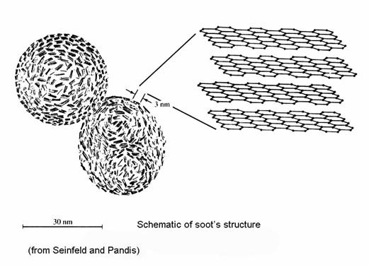
Elemental carbon, or soot, is formed when C/O ratios in combustion are greater than 0.5. As fuels are oxidized in flames, they are broken down into smaller molecules, including acetylene (C₂H₂) and polycyclic aromatic hydrocarbons (PAHs). Soot nuclei are formed, and then gas-phase polymerization adds more carbon mass to the nuclei until soot particles are formed. Soot particles grow to about 10 nm, and then coagulate to form chain aggregates.

Soot formation depends on the ratio of carbon to oxygen in the combustion process of hydrocarbons. If there is insufficient oxygen to convert all the carbon to CO₂ from a fuel C_mH_n, then the stoichiometry is:

C_mH_n + a O₂ ® 2 a CO + 0.5 n H₂ + (m-2a) C_s

C_s is the soot that is formed and the carbon/oxygen ratio, C/O, is m/2a. When m = 2a, C/O = 1 and all the carbon will be tied up as CO and no soot will be formed. If even more oxygen is available, then some of the CO will be converted to CO₂. Because some CO and CO₂ is always formed in combustion processes, soot will form even when C/O is less than 1. It has been experimentally determined that soot can start to form for C/O as small as 0.5.

The tendency to form soot depends on the type of chemical compound. Multi-ring compounds, like naphthalene, form more soot that benzene, a single ring compound, which forms more soot than alkenes, alkanes, and alkynes. Diesel engines, furnaces burning rich, and fireplaces are the principle sources of soot.

Elemental carbon concentrations range from 0.2 to 2.0 mg m^-3 in rural areas to 1.5-20 mg m^-3 in urban areas. Sizes range from 0.1 to 1 mm diameter.

Organic carbon consists of thousands of organic compounds. Typically, organic carbon masses are reported for the carbon mass only and do not include the mass of other chemicals, such as hydrogen, nitrogen, and oxygen. Organic carbon is found to be 0.1-1 mg(C) m^-3 in remote areas to ~4 mg(C) m^-3 in rural areas to 5-20 mg(C) m^-3 in urban areas.

The size distribution is typically in the nucleation and the accumulation modes from 0.1 to 1 mm diameter.

Primary organic carbon. The primary organic carbon emitted in LA consists of:

• meat cooking (21%)
• paved road dust (16%)
• fireplaces (14%)
• non-catalyst cars (12%)
• diesels (6%)
• surface coatings (5%)
• forest fires (3%)
• catalyst-equipped vehicles (3%)
• cigarettes (3%).

The chemical composition of primary organic compounds is typically C-10 and higher compounds. The size is typically 0.1-1 mm diameter.

Secondary Organic Carbon (SOC), or Secondary Organic Aerosol (SOA).

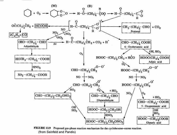
The aerosols are produced when organic compounds are oxidized and some oxidation products have very low vapor pressures. The following figure shows the proposed pathways for cyclohexene (C₆H₁₀) oxidation by ozone. Note the formation of several acids as well as aldehydes.

Precursor gases for secondary aerosol formation.

The ability of a volatile organic compound to form secondary aerosols depends on three factors:

1. its atmospheric abundance;
2. its chemical reactivity;
3. the volatility of its products.

In many cases, VOCs meet the first two criteria, but its products are volatile. Methane (CH₄) is an example. Its products – CO, HCHO, CO₂ – are all volatile with high vapor pressures.

Secondary organic aerosols are generally produced from the chemical types:

• alkanes with more that 6 carbons;
• alkenes with more than 6 carbons;
• polycylclic aromatic hydrocarbons (PAHs).

Low-molecular weight alkanes, alkenes, aromatics (like benzene), and carbonyls (like acetone), chlorinated chemicals and oxygenated solvents do not produce secondary organic aerosols.

An interesting class of VOCs that can form secondary organic aerosols are the biogenic VOCs. While oxidation of isoprene (C₅H₈) does not contribute to SOA formation, oxidation of some monoterpenes (C₁₀H₁₆) and sesquiterpenes (C₁₅H₂₄) can. Relatively little is known about these biogenic emissions. There is growing evidence that many terpenes of some type have not been observed but are influencing SOA formation, O₃ destruction, and OH production.

The typical low-vapor pressure product gases that form secondary organic aerosols include high molecular weight acids and nitrates.

In Los Angeles, the contributions of different hydrocarbon classes to SOA formation are the following:

aromatics (~60%), biogenic hydrocarbons (~10-15%), alkanes (15-20%), and alkenes (5-10%).

Transfer of low-vapor-pressure gases between the gas and aerosol phases.

We will quantify the process by several different measures: mass concentration, mass fraction in the aerosol phase, and yield in the aerosol phase.

Noninteracting Secondary Organic Aerosol Compounds.

The mass transfer of these products to the aerosol occurs if the gas-phase concentration is larger than the equilibrium gas-phase concentration:

J = c_g - c_eq

where c_g is the concentration in the gas phase and c_eq is the equilibrium concentration in the gas phase.

If c_g > c_eq, then the atmosphere will be supersaturated with the organic compounds. Thus, to find the organic compounds that are likely to form SOA, we need to look at compounds with low vapor pressures relative to their likely gas-phase production.

The following figure shows the behavior of adipic acid as a function of time. Adipic acid comes from the oxidation of cyclohexance. c_eq = 0.08 ppb. If the mixing ration of adipic acid exceeds 0.08 ppb, then the rest will go onto an aerosol.

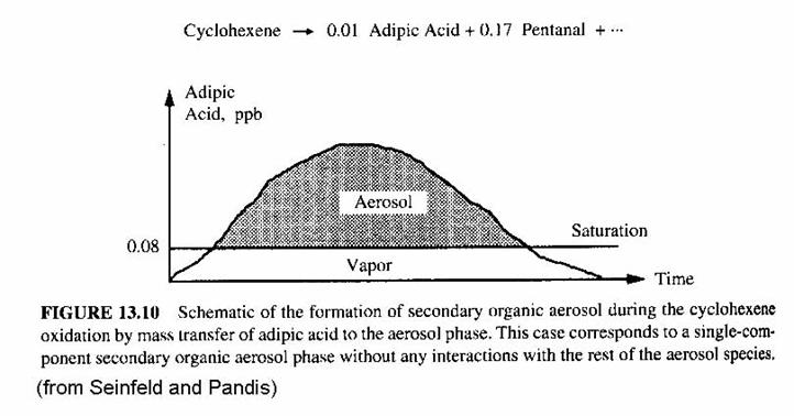
This case is an idealized case. The chemical has not be dissolved in the aerosol, as happens with the aqueous chemistry that we have previously discussed; nor has it been adsorbed, which requires chemical interactions with the molecules on the aerosol’s surface.. In this simple, idealized case, the reactive organic gas does not interact with the molecules on the aerosol’s surface.

ROG = reactive organic gas.

ROG ® S_i a_i P_i, where a_i is the yield of product P_i from the ROG. For example the reactive organic gas may react with OH and the resulting product of the oxidation sequence is a low vapor pressure organic acid.

The total mass concentration, or mass density, of a product chemical, P_i, is: c_t,i = c_g,i + c_aer,i. All have units of mg m^-3 of air.

At equilibrium, c_g,i = c_eq.i = p_i^oM_i/RT, where we use the Ideal Gas Law and M_i is the molecular weight of the molecule, p_i^o is the equilibrium vapor pressure if chemical species i.

For c_t,i < c_eq,i , then c_aer,i = 0 . In this case, none of chemical species i is in the aerosol.

For c_t,i > c_eq,i, c_aer,i = c_t,i – c_eq,i. Now, the equilibrium value of the mass concentration, which is of course related to the vapor pressure, has been exceeded and some of the chemical species i is now deposited on the aerosol. As c_t,i increases, more of chemical species i goes into the aerosol.

Let’s relate these concentrations to the change in concentration of the reactive organic gas, DROG.

The total concentration = DROG, in mg m^-3.

c_t,i = a_i (M_i/M_ROG)DROG.

The middle term normalizes c_t,i for mass difference between the ROG and the oxidation product because we are using mass-based units, not number-based units.

Therefore, c_aer,i = 0 if DROG < DROG_i* , which is the threshold value for DROG.

c_aer,i = a_i (M_i/M_ROG) DROG – c_eq,i if DROG > DROG*.

The threshold ROG change is given by the equation:

DROG_i* = (p_i^oM_ROG)/(a_i RT)

since

c_eq,i = p_i^oM_i / RT = a_i (M_i/M_ROG) DROG*

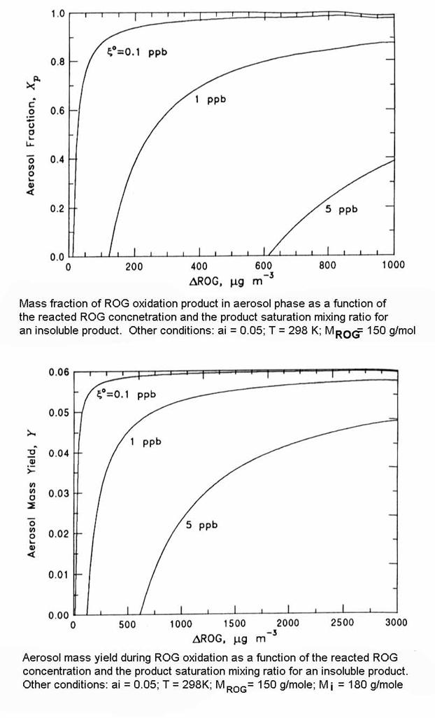
Let’s add some new definitions. X_p,i = mass fraction in the aerosol phase: X_p,i = c_aer,i / c_t,i .

X_p,i = 0 if DROG < DROG*

X_p,i = 1 – (p_i^o M_ROG)/(a_i RT DROG) = 1 – (DROG*/DROG), if DROG > DROG*.

We are interested in knowing what the aerosol mass yield is for different reactive organic gases. The yield, Y_i, is defined as:

Y_i = c_aer,i / DROG

Y_i = 0 if DROG < DROG*

Otherwise, if DROG > DROG*,

Y_i = a_i (M_i / M_ROG) – (p_i M_i)/(RT DROG) = (c_aer,i a_i M_i RT)/(c_aer,i RT + p_i^oM_i)M_ROG

Formation of Binary Ideal Solution with Preexisting Aerosol - Dissolution.

In this case, we assume that the chemical species is partitioned according to Henry’s Law. The aerosol component of species i starts to grow as soon as the particle is formed, unlike the previous case, where the aerosol phase occurred only when the gas phase partial pressure exceeded some value.

Define m_o = pre-existing aerosol mass (mg m^-3) and M_o = molecular weight of pre-existing aerosol molecule.

The mole fraction of the chemical species in the aerosol phase is given by:

x_i = (c_aer,i / M_i) / (c_aer,i / M_i + m_o / M_o)

For an ideal solution that obeys Henry’s Law, the vapor pressure p_i is equal to the mole fraction x_i times the vapor pressure for the pure solution of chemical species i:

p_i = x_i p_i^o

Putting this in mass units (mg m^-3),

c_g,i = (x_i p_i^oM_i) / RT

Combining these three equations by eliminating x_i and c_g,i , we obtain the expression:

But, usually c_aer,i << m_o.

From these equations, we can also derive the mass fraction of i in the aerosol phase:

and the aerosol mass yield of the ROG:

Adsorption and gas/particle partitioning of organic materials.

Aerosols can absorb gas molecules on their surfaces. Absorption involves both microphyics and chemistry. As adsorption occurs, a partial covering becomes a more complete monolayer. Once new gas molecules can be adsorbed only onto the monolayer of the same chemical to form a multi-layer, the chemical properties and adsorption process can change.

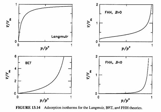
An absorption isotherm – the dependence of the amount of gas adsorbed at a constant temperature – is used to characterize the adsorption. The most common is the Langmuir isotherm for a equilibrium adsorption of a monolayer, which has the following assumptions:

1. All surface adsorption sites are equivalent.

2. Adsorbed molecules do not act horizontally.

3. All molecules have the same heat of adsorption for any site.

The Langmuir isotherm has the form:

where V is the volume of gas adsorbed at equilibrium at gas partial pressure p, V_m is the gas volume that will form a monolayer, and b is a constant that depends on the surface properties of the adsorbing material.

The BET theory extends the Langmuir isotherm concept to multiple layers. It uses the assumptions:

1. An absorbed molecule in one layer can be a site for adsorption in the next layer.
2. The heat of adsorption is equal to the latent heat of evaporation for the bulk condensed gas for all adsorbed layers except the first layer.

where S = p/p^o is the gas-phase saturation ratio, as we introduced before, p is the adsorbing gas’ partial pressure, p^o is the adsorbing gas’ saturation pressure, and c is a constant that is different for different surfaces. Unfortunately, BET predicts infinite adsorption if p = p^o.

Perhaps a better isotherm is the FHH isotherm, which is given by the expression:

where A and B are constants for the adsorbing surface. The behavior of the various isotherms with respect to S can be seen in the figure below. All three of these theories require experimental data to determine the constants for each surface type and each adsorbing gas.

The typical behavior of the different isotherms is given in the figure below.

Vapor adsorption on particles is typically defined by a partitioning coefficient, which indicates the partitioning of the chemical species in the gas and particle phases. This partitioning coefficient is given by the expression:

where K_p is the temperature-dependent partitioning coefficient in m³ mg^-1, M_t is now the total ambient aerosol mass concentration in mg m^-3, and c_aer and c_g are the aerosol and gas mass concentrations in mg m^-3. The greater the aerosol mass, M_t, the more of the gas that can be adsorbed onto the particle. A larger K_p implies that more of the chemical species will be adsorbed onto the aerosol.

For purely physical adsorption, the partitioning coefficient K_p can be found with the expression:

where N_s is the surface concentration of sorption sites (sites cm^-3), a_s is the aerosol’s specific area (m² g^-1), Q_l is the enthalpy of desorption from the surface (kJ mol^-1), Q_v is the enthalphy of vaporization of the chemical as a liquid (kJ mole^-1), R is the gas constant, T is the temperature (K), and p^o is the vapor pressure of the chemical as a liquid (hPa).

Laboratory researchers have tried to fit this expression with an equation of the form:

where m = -1 and b_r = -7.8 for polycyclic aromatic hydrocarbons (PAHs) and b_r = -8.5 for organochlorines.

The temperature dependence of K_p is given by the expression:

where A_p is a constant that depends on the chemical.

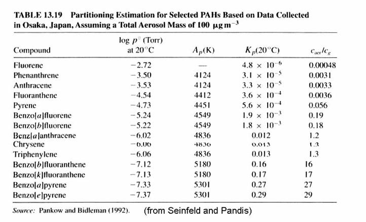
The coefficients for selected PAHs are provided in the following table.

Chemical composition: a summary.

The typical chemical composition of aerosols can be seen in the following table and figure.

Some typical aerosol composition fractions are:

average urban fine (33mg m^-3)		average remote fine (5 mg m^-3)
species	percent	species	percent
SO4	28	SO4	22
NO3	6	NO3	3
NH4	8	NH4	7
C-elem	9	C-elem	0.3
C-organic	31	C-organic	11
unknown	18	unknown	57

We can also see the two most important characteristics of aerosols – size distribution and chemical composition – in the following figure.

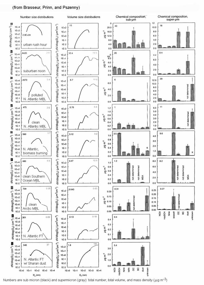
We see that there are a wide range of aerosol number and mass concentrations, and quite different number and volume size distributions. We will see the importance of these differences when we discuss atmospheric chemistry and climate in Chapter 8.