3.1 Actinic flux

3.1.1 Energetics

Energy from the Sun drives atmospheric chemistry by exciting atoms and molecules to higher energy states and by breaking chemical bonds. For these processes to happen, atoms and molecules must be able to absorb the solar radiation.

Radiation energy is given by E = hn, where E is the energy in Joules, h is Planck's constant (h = 6.626x10^-34 J s), and is the frequency of the light in units of s^-1. Frequency is related to wavelength by l= c/n, where c, the speed of light, is 3.0x10⁸ m s^-1. Another unit that you will often see is wavenumber, = 1/l, and has units of cm^-1.

We can think of light either as waves or as individual particles called photons. The energy of a single photon of wavelength is given by:

E = hc/l = (1.98x10^-16/ (nm)) J photon^-1,

where l is in units of nm. Note that 1 Joule = 6.242x10¹⁸ eV, 1 cal = 4.184 J. If we consider the amount of energy as distributed in a mole of gas, we get the relationships:

1 eV = 23.06 kcal mol^-1 = 96.48 kJ mol^-1 = 1.60x10^-19 J molecule^-1

3.1.2 The solar spectrum

The Sun emits acts as a black body. The distribution of energy over wavelengths is given by the expression for the monochromatic emissive power:

E(l)= {2pc²hl^-5}/{exp(ch/klT) - 1}

For a black body, the wavelength of peak emission is found from the equation:

l_max(nm) = 2.897x10⁶ /T(K)

The Sun has an effective radiating temperature of 6000K, so that the wavelength of peak radiation is near 500 nm. The total energy from the Sun is given by the Stefan-Boltzmann Law:

E_B = ∫E(l)_Bdl = sT⁴

where s= 5.67x10^-8 W m^-2 K^-4, the Stefan-Boltzmann constant. The Sun is not a perfect blackbody, however, as seen in Figure 3.1.

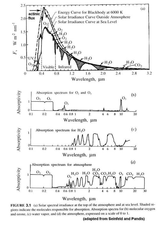
The quantity of interest for atmospheric photochemistry is the actinic flux, which is the radiative flux from all directions. It is related to the solar irradiance, which is the amount of solar energy that strikes a unit surface area per unit wavelength. Whereas the solar irradiance depends on the angle between the sun and the normal to the surface, the actinic flux remains the same. If we shrink our volume down to the size of a molecule, then we can see that it does not matter the angle at which that molecule is struck. The solar irradiance integrated over all wavelengths is called the solar constant, S, and S = 1367 W m^-2 when the Earth is 1 AU (astronomical unit) from the Sun.

The solar irradiance changes over the course of a solar cycle. This change is at most a few percent for the solar constant, but is as much as several 10's of % for wavelengths less than 300 nm. The actinic flux likewise changes over the course of the solar cycle. The changes can be large for the mesosphere, but are not particularly large for the troposphere.

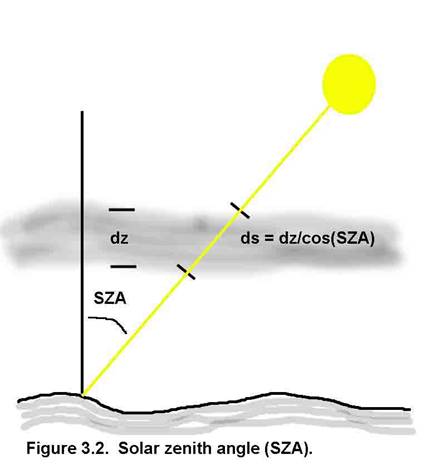
Up to now, we have dealt with the amount of light at the top of the atmosphere. What we are interested in is the amount of light that is incident on a particular volume of air from the surface to the top of the stratosphere. The amount of light in that volume may be different from the light at the top of the atmosphere because of absorption and scattering. A major factor is the solar zenith angle (SZA), as shown in Figure 3.2. As the solar zenith angle increases, the total path through an absorbing layer also increases, thus reducing the energy that arrives at any volume of air below the absorber.

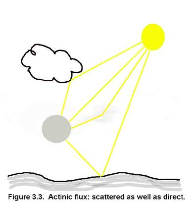
Absorption and scattering can reduce the amount of light, but scattering can also increase the amount (Figure 3.3). So, for actinic flux, it does not matter from which direction the energy comes, as long as the energy spectrum is not modified.

The units for actinic flux are typically not W m^-2, as is the irradiance. If we think about what is happening at a molecular level, a photon strikes the molecule and its energy is absorbed. What happens next depends a lot on the energy of the photon and the type of molecule or atom, but we can write the interaction as if the photon was a chemical, (e.g., AB + hn ® A + B). Thus, the logical units for actinic flux are photons cm^-2 s^-1. Just like the irradiance, the actinic flux varies with the sun’s solar spectrum. The spectral actinic flux, which is the amount of actinic flux in a given wavelength interval, has the units of photons cm^-2 s^-1 nm^-1; it is shown in Figure 3.4 for different altitudes.

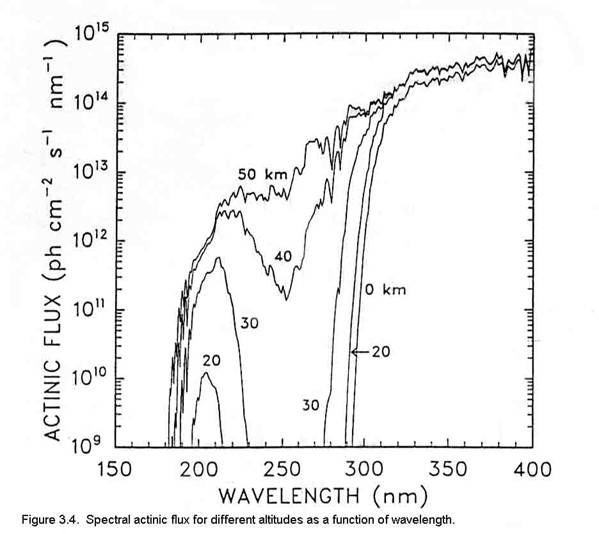
As is shown in Figure 3.1, the actinic flux below about 180 nm is decreased by strong absorption of solar energy by molecular oxygen. The large decrease in actinic flux between 220 and 300 nm is due to ozone, which is predominantly in the stratosphere. Note the very rapid increase in actinic flux near 300 nm. The bond strengths of hydrogen-carbon bonds in many organic molecules is about 60 to 120 kcal mole^-1. Since the energy of a photon at 300 nm is ~95 kcal mole^-1, increasing the actinic flux in this spectral region has the potential to break more organic chemical bonds.

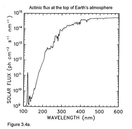
The actinic flux at the top of the atmosphere is shown in Figure 3.4a. Comparing this figure to Figure 3.4 illustrates the effects of O₂ absorption high in the atmosphere.

3.2 Simplified spectroscopy

We can understand a molecule’s absorption spectrum by using quantum mechanics. Atoms and molecules are held together with electrical forces. Particularly important is the attraction of opposite charges and the repulsion of like charges. The attraction and repulsion of charges do a balancing act that results in the structure of atoms and molecules. By adding energy to the atom or molecule, it is possible to separate the charges and let them establish a new arrangement. We can add energy with heat or with radiation.

Another factor is that atoms and molecules can make only discrete changes in energy. This quantitized energy results from Bohr's postulate that the angular momentum of the electron around an atom could take only quantitized values. Quantum theory has been very successful in describing the observed absorption of atoms and molecules, and so, we will use it in the following discussions to get an idea about why atoms and molecules absorb the light that they do.

Electrostatic forces attract the negative-charged electrons to the positively charged nucleus. The force between the electrons and the nucleus is:

F = q₁q₂/r² giving electrostatic potential energy E = ∫F dr = - q₁q₂/r

Thus, a nucleus of total charge q₁ will attract enough electrons with a total negative charge of –q₁.

The Bohr atom. Assume that an atom has Z protons. The force on an electron is Ze²/r², so that Ze²/r² = m_ev²/r, or r = Ze²/m_ev². Bohr postulated that the angular momentum of the electron must be a multiple of h/2p, so that m_evr = mω = n h/2p, where h is Planck’s constant = 6.625x10^-34 J s, m_e is the electron’s mass = 9.11x10^-31 kg, v is the electron’s velocity, r is the radius of its orbit, and ω is its angular velocity. So eliminating the velocity from the equation for r, we find that:

These orbits may be elliptical, not circular, however.

The energy of the electron in the orbit is a sum of the potential energy and the kinetic energy. The potential energy is the integral over r of the force and is equal to –Ze²/r, while the kinetic energy is equal to ½ m_ev² = Ze²/2r. Thus, the total energy is given by the expression:

Applying Bohr’s quantitization, the energy for any quantum number n is given by the expression:

Bohr further postulated that photons could be absorbed or emitted only if their energy matched the separation between energy levels of the electron:

Although Bohr approached the problem assuming that the electrons were particles, it is also possible to approach the problem assuming that the electrons can be represented by waves. This leads to the time-independent Schroedinger Equation:

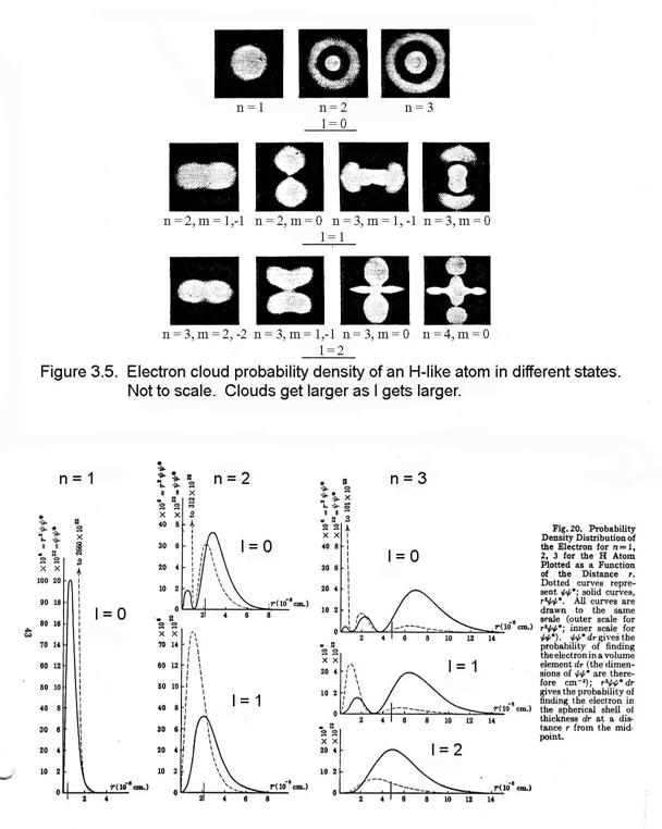
where E is the total energy, V is the potential energy, and Ψ is the electron’s wave function, which resembles an electron cloud.

For atoms, this differential equation is usually solved in spherical coordinates. In the process of separating the radial and angular functions, variables of separation emerge. At the same time, the solution for the wave function emerges as a radial function and angular wave functions.

If in the course of circling the nucleus the electron’s wavelength is too long or too short to repeat from cycle to cycle, the wave will interfere destructively with itself and rapidly die out. Hence, for the wave to remain, its wavelength must be such that an integral number of them occur in one revolution around the nucleus: 2πr_n = nλ, where n = 1, 2, 3, … de Broglie postulated that all matter has a wave nature and that the wavelength of a particle is given by the expression: λ = h/mv. Thus, substituting this expression into the previous one, we find that mvr_n = nh/2π, which is exactly Bohr’s assumption about the angular momentum being quantititzed.

Thus, because of this quantatization of angular momentum, the constants of separation can take only certain values. To describe the electron’s wave requires four quantum numbers, which are these separation variables, as in Table 3.1

Table 3.1. Electron quantum numbers
name	symbol	possible values
principal	n	1, 2, 3, …
orbital	l	for a given n, l can be 0, 1, 2, …, n-1.
magnetic	ml	for a given n and l, ml can be l, l-1, …, 0, …, -l.
electron spin	ms	for each set of n, l, ml, ms can be +1/2 or -1/2.

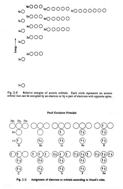
Pauli proposed that no two electrons in an atom can have the same set of 4 quantum numbers. This Pauli Exclusion Principle provides the quantum mechanical foundation for the periodic table of the elements.

The innermost orbital is spherical and is called the s-orbital. The n=1 energy level can have only an s orbital. It can contain 2 electrons only (by the Pauli Exclusion Principle), which have the same n, l, and m_l, but different m_s. The next quantum level for angular momentum, called the p-orbitals, are shaped like dumb-bells and can hold 6 electrons, since for any value of l, there are 2(2l+1) possible values of m_l and m_s. The n=2 energy level has both s- and p- orbitals and is filled with 8 electrons. The next angular momentum level, called the d-orbitals, have a variety of shapes and can hold 10 electrons. The n=3 energy level has s-, p-, and d- orbitals and is filled with 18 electrons. Figure 3.6 shows the relative energy levels for the different electrons.

Atoms are stable with filled shells, such as helium (atomic number =2), neon (atomic number =10), and argon (atomic number = 18). Atoms that have partially filled shells either have a tendency to give up or take electrons from other atoms. The atoms that are given up or taken are in the highest energy levels for the atom, and are called the valence electrons. The innermost electrons do not participate in chemical reactivity because they fill complete shells and they partially shield the outer electrons from the nucleus. The weakest bond is for atoms with only one electron in the other shell, such as lithium (a.n. = 3), sodium (a.n. = 11), and potassium (a.n.=19). The atoms with the greatest affinity for electrons have just one electron missing to complete a shell, such as hydrogen (a.n.=1), fluorine (a.n.=7), and chlorine (a.n.=17).

The ionization potential is the energy required to remove an electron from an atom. For Na ® Na⁺ + e^- , IP = 5.1 eV = 8.2x10^-19 J

The ionization potentials for the alkali atoms (Li, Na, K) are quite low, typically 5 eV; the ionization potentials for the halogen atoms are typically quite high 13-16 eV. Noble gases have even higher ionization potentials.

Some atoms with incomplete shells will take up an extra electron even though they then have a negative charge. This is called electron affinity.

The tendency for atoms to attract electrons is called electronegativity (Pauling). The halogens have the greatest electronegativity (Fluorine is 4.0) while the alkalis have the least (Potassium is 0.8). The ionization potential and the electronegativity of various atoms can be used to try to predict the types of molecular bonds that form and how strong they will be.

Designation of ground and excited state atoms. In general, it is only the outermost electrons that are involved in chemical reactions and in absorption and emission of photons. The total angular momentum, L, equals the sum of the angular momenta of individual electrons in the outermost shell: L = l₁ + l₂ + …. L=0, 1, 2, 3, 4, … are designated by the capital letters S, P, D, F, G, … respectively. The total electron spin, S, is the sum of the electron spins of the individual electrons in the outermost shell: S = m_s1 + m_s2 + … The value 2S+1 is called the multiplicity, because electrons with the same n and l but different m_l are at the same energy level (except when put in a magnetic field). Because individual electron angular momenta and electron spin can have a range of values each, the electrons in an atom have a number of possible values of S and L.

The energy level of the electrons in the atom can be uniquely defined by ^2S+1L.

For instance, oxygen has 8 electrons, 2 in the 1s orbital, 2 in the 2s orbital, and 4 in the 2p orbital. They are distributed as in Figure 3.6b. Of all the possible states – ¹D, ³P, and ¹S - Hund’s Rule says that the state with the highest multiplicity lies lowest and of states with the highest multiplicity, the one with the greatest L lies lowest. So, the ground state of the oxygen atom is the ³P state.

When atoms absorb energy equal to the separation between energy states, electrons can be promoted from the lower energy level to a higher energy level. However, because electron spin and angular momentum must be conserved in the transition, not all transitions are possible between the states. In fact, only transitions with DS = 0 and Dl = ±1 are allowed. These rules can be violated, but the “forbidden” transitions take a lot longer to occur.

Molecular structure

Atoms can form different kinds of molecular bonds. We will start talking about diatomic molecules first because they are easiest.

Ionic bonds. For atoms with highly different electronegativities, the atom with low electronegativity (the electron donor) gives up an electron, becoming a positive ion. The atom with high electronegativity takes up the electron, becoming a negative ions. The two ions attract each other and form a molecule. There is essentially a complete transfer of the outermost, or valence, electron from one atom to the other. An example of this is NaCl.

Covalent bonds. When two of the same atoms with fairly high electronegativities or two different atoms of similar electronegativities get together, it is possible for them to share electrons and form a chemical bond. These shared electrons can spend some time between the two nuclei, thus helping to bond the molecule together. Most organic molecules and many inorganic molecules are held together with covalent bonds.

The typical bond strength of atmospheric molecules is from about 2 to 8 eV. We will see how this affects the absorption in the atmosphere after we look at a little diatomic spectroscopy.

What determines how far apart the two nuceli are from each other. We have two electrostatic forces at work. At great distances, the two nuceli are attracted by the negative charge of one and the positive charge of the other. As they get very close though, the electrons are squeezed out from between the positive nuclei and the two positively charged nuclei repulse each other. This can be seen with an energy diagram, where r is the separation of the nuceli and E is the energy of the total system. The most stable position is that which has the least amount of energy. The resulting energy curve is called the Morse potential (Figure 3.7).

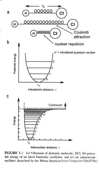
However, the minimum in the Morse potential is not the minimum in the actual energy of the diatomic molecule. Diatomic molecules vibrate; diatomic molecules rotate. Thus, within the Morse potential are quantitized levels of vibration and rotation.

The energy of the vibrational levels is given by the equation:

where h is Planck’s constant, n_vib is the vibrational frequency that depends on the spring constant of the chemical bond, x_e is the anharmonic constant and n is the vibrational quantum number = 0, 1, 2, …. Note that as n increases, the anharmonic term becomes more important – the separation between energy levels decreases. For interactions with infrared radiation, the selection rule is that Dn = ±1 for allowed transitions, although the anharmonic term enables changes of ±2, ±3 to occur in what are called overton bands.

The molecule can rotate as well as vibrate. These rotations are quanitized, just as the vibrations are. The energy levels associated with rotations are given by the expression:

where I is the moment of inertia = mr² and J is the rotational quantum number = 0, 1, 2, …. For interactions with far infrared radiation, the selection rule for the rigid rotator is DJ = ±1. The energy between consecutive energy levels is given by DE_r = 2B J’, where J’ is the quantum number of the upper of the two levels.

Diatomic molecules have several possible energetic transitions. They can move, or translate; they can vibrate; they can rotate; and the electrons can change energy levels, similar to atomic electronic transitions. Typical energy ranges for these different possible energy changes are in Table 3.2. Translational, rotational, and vibrational energies are insufficient to break most chemical bonds. Thus, we will focus on electronic transitions.

Table 3.2. Energy of diatomic transitions
transition	energy range
translation	0.03 eV; 50 cm^-1
rotation	2x10^-4 eV; 2 cm^-1
vibration	0.5 eV; 5000 cm^-1
electronic	5 eV; 50,000 cm^-1

Most molecules will tend to be in the lowest vibrational and rotational quantum levels. The distribution in these energy levels is controlled by the Boltzmann probability distribution function. For vibrations, we have the expression:

Similarly, the rotational distribution is given by the expression:

N₀ is the number of molecules in the J=0 level. We must multiply by (2J+1) because there are (2J+1) ways combine orbital angular momentum and spin. This is called a degeneracy. Note that B is in units of wavenumbers (cm^-1), so that the energy of the rotation is obtained by multiplying by h (6.63x10^-34 J s) and the speed of light (3x10¹⁰ cm s^-1). The Boltzmann constant, k, is 1.38x10^-23 J K^-1.

We see that in both cases, molecules will be distributed in more than one level. For vibrations, most molecules will be distributed in the lowest vibrational level, v”=0, but some will be in the v”=1 and less in the v”=2 levels. It all depends on how large n_vib is. For rotations, most molecules may not be distributed in the lowest level because of the degeneracy factor. Also, since B ~ kT, we can expect that molecules will populate many more rotational levels than vibrational levels.

Electronic transitions.

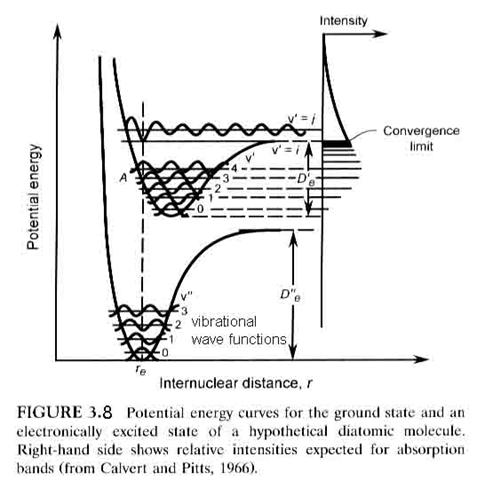
So far, the discussion has focused on the ground electronic state of a diatomic molecule. However, when an electron is promoted to a higher orbit in the molecular electron cloud, the molecule can still be bound by the chemical bond and will still vibrate and rotate. Usually, the internuclear distance increases and the molecular energy is higher, as seen in Figure 3.8. Note that it is possible for the excited molecule to be stable and not decompose if it is elevated to a bounded excited state. Depending on the molecule and the state, the excited state molecule will usually give off a photon and return to the ground state within nanoseconds to microseconds. It is also possible that the molecule will be promoted to an unbound state, in which case, the molecule will fall apart on the next vibration into two atoms, although one of them may be excited. A photon must have enough energy to excite the molecule to a level that is greater than D”_e, however, if the molecule is going to dissociate.

Just as there are selection rules for vibrational and rotational transitions, there are selection rules for electronic transitions.

· DS = 0, where S is the sum of all electron spins. Just as for atom, 2S+1 is called the multiplicity.

· DΛ = 0, ±1, where Λ is the component of the electronic orbital angular momentum that lies along the internuclear axis.

· DJ = -1, 0, +1, where J is the rotational angular momentum quantum number. DJ = -1, 0, +1 are denoted as the P, Q, and R branches respectively.

· u ↔ g, but no u ↔ u or g ↔ g, where u and g are the wave function symmetries when reflected through the center of the molecule.

· ⁺ ↔ ⁺ or ^- ↔ ^-, but not ⁺ ↔ ^-, where these superscripts denote the wave function symmetries when reflected through the plane passing through the two nuclei.

Electronic states are designated by a letter – typically X, A, B, C, …, which designates the electronic state (X is used for the ground state), and the expression: ^2S+1 Λ, where Λ=0, 1, 2, 3, 4, .. is denoted by S, Π, Δ, Φ, … respectively.

There is one more principle that determines which transitions can occur – the Frank-Condon Principle. The basic idea is that when an electron jumps from one electronic state to another, it does it much faster than a molecular vibration. The atoms in the molecule remain at the same internuclear distance while the electronic transition occurs. 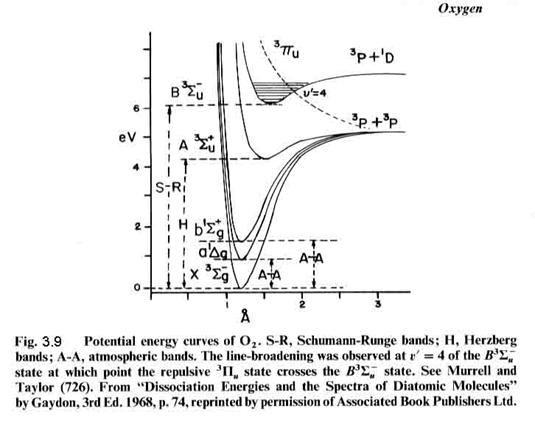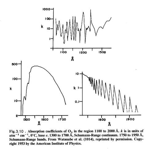This means that the only electronic transitions that can occur are those that can be connected by a straight vertical line, as shown in Figure 3.8. Molecular absorption is directly linked to the energy levels of the molecule, as seen for molecular oxygen in Figures 3.9 and 3.10. For instance, the S-R bands (Schumann-Runge) overlap with a repulsive state (no minimum) at v’=4, which has an energy of about 6.6 eV, which corresponds to a photon with a wavelength of ~190 nm. We can see the absorption just starting as bands in the lower right absorption curve. The bands give way to a continuum at about 1750 nm, where production of ³P and ¹D oxygen atoms is possible (but may not occur frequently).

Polyatomic molecules. The same basic concepts apply to polyatomic molecules as to diatomic molecules. However, things get much more complex because the molecules have 3n-6 vibrational degrees of freedom for a non-linear molecule, like H₂O, where n is the number of atoms, and 3n-5 vibrational degrees of freedom for a linear polyatomic molecule, like CO₂. In addition, there is much more interactions among the various states, so that overtone bands and combination bands (coupled vibrations) are much more frequent.

3.3 Beer-Lambert Law and relationship to spectra.

Suppose we have a volume of gas that absorbs. Then, in an infinitesimal slab of that medium, a certain fraction of the light with irradiance I, called dI is absorbed. dI is equal to the probability of absorption, called the cross section (cm^-2), the number density of the absorbers, and the length of the light-path through the slab, dl:

dI = I s n dl.

Integrating this expression over the total thickness of the volume, we get the Beer-Lamert Law:

I = I_o exp (-s n l),

where l is the length of the light path through the volume. Sometimes, this we substitute a variable k for s n. In fact, you will see the absorption coefficient reported a large number of ways.

Once we know the absorption coefficients of all of the absorbing molecules between the sun and the air volume of interest and the number densities of the absorbers, we can determine how much light will be absorbed at every wavelength.

The angle of the Sun with respect to the zenith (directly overhead) affects the total path through absorbers, and thus is important.

The result is that we can write dl = (1/cos(SZA)) dz = sec(SZA) dz in the differential form of Beer's Law:

dI/I = n sec(SZA) dz,

or I(z) = I_infinity exp(- ∫sec(SZA) s_z n(z) dz)

Usually, but not always, s is not a function of altitude. It sometimes is because it is a function of pressure and temperature, which vary for different altitudes.

3.1.3 Photolysis frequencies.

Photochemical reactions.

When molecules absorb light (called photolysis), several processes can occur:

1.Dissociation: A + hn --> C, where A is the absorbing molecule,  hn is the typical symbol for light, and B and C are products of the dissociation.
2.Reaction: A +  hn  --> A* + B --> C + D, where A* is an excited state molecule or atom.
3.Fluorescence: A +  hn --> A +  hn' where  hn' may be different from  hn.
4.Collisional deactivation: A +  hn --> A* + M --> A + M, with the energy going into heat.

Photolysis frequencies.

The photochemical reactions written above can be described quantitatively using rate equations.  The rate equation for photolysis is:

d[A]/dt = - J [A].

J is a first-order rate constant and is a special kind of rate coefficient that we call the photolysis rate coefficient. If this is the only
process happening to chemical species A, then in out usual fashion, we can find the change in [A] with time, and it is:

                                                                 [A] = [A]_o exp (- J t ).

where [A] is the concentration of chemical A at time t, [A]_o is the concentration of A at t=0. What determines J for a given volume of air? It depends on the actinic flux at that volume, the absorption cross section of A as a function of wavelength, usually denoted by s, the absorption cross section, and the quantum yield of the process, designated by j. When a molecule absorbs energy, it is possible that more that one result can occur. The quantum yield is the fraction of time that when a photon is a absorbed a particular result will occur. Thus,

                                                             J = ∫ F(n)T(n)s(n) j(n)dn

where the spectral actinic flux, F, has units of photons cm^-2 s^-1 nm^-1, the atmospheric transmission to the volume of air, T, is unitless, the absorption cross section, s, has units of cm² per molecule, and the quantum efficiency, j, is a fraction and thus unitless. The resulting photolysis frequency has units of s^-1, which is exactly what a frequency is. Sometimes J is called a photolysis rate, but photolysis frequency is more unambiguous.

We can also do the integration over a wavelength range as well as a frequency range.  Also note that the photons can reach the volume of air not only directly from the sun, but also from reflections from clouds or the ground.  Photolysis has been observed to increase a factor of two or more for some situations where there are clouds below.

We can estimate the terms in the integral for J in order to determine the importance of a photochemical reaction. Consider the molecule NO₃, the nitrate radical by looking in the JPL kinetics book.  It absorbs mostly between 600 and 670 nm, and has a lumpy absorption cross section, but the rough average is about 5x10^-18 cm². The solar irradiance is in this wavelength range is about 5x10¹⁴ photons cm^-2 s^-1 nm^-1, or about 3.5x10¹⁶ photons cm^-2 s^-1. For the photodestruction of NO₃, j=1.

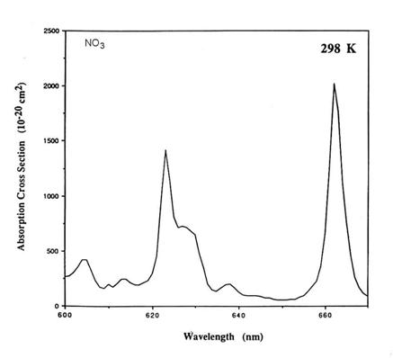
Thus,

                                                         J = 5x10¹⁴ 5x10^-18 1 70 = 0.18 s^-1

1/J is a characteristic time scale for the photodestruction of NO₃, often called a lifetime.

The correctly calculated photolysis rate coefficient is slightly more than 0.2 s^-1. So our estimate is close.

3.1 Chemical kinetics

Most photochemical models of the stratosphere contain about 35 different chemical species and about 160-200 individual reactions. The reaction rate coefficients for these reactions were carefully measured in the laboratory and are accumulated in the JPL rate handbook (http://jpldataeval.jpl.nasa.gov/pdf/JPL_02-25_rev02.pdf). You should download this onto your computer.

3.1.2 Reaction energetics

Which reactions happen?

Suppose that we think of a reaction: NO₂ + O₃ ® NO₃ + O₂. How do we know that this reaction actually happen?. What do we need to know to find out?

This most important, but not only criterion, is that the reaction acts to lower the enthalpy of the reaction. Recall that the definition for enthalpy is given by the equation:

H = E + PV

where H = enthalpy (kJ mole^-1), E is the internal energy, and P and V are pressure and volume respectively. For a constant pressure process, the change in the enthalpy is given by:

DH =DE + pDV = heat absorbed

The DH values for a large number of molecules is given in the JPL document, starting on page 325.

For the reaction of NO₂ with O₃, we need to know if the enthalpy of the reactants (NO₂ and O₃) is greater or less than the enthalpy of the products (NO₃ and O₂). If the enthalpy of the products is larger than that of the reactants, then extra energy is required to make the reaction occur, as shown in the figure. The reactions always want to run downhill, to lower enthalpy. Thus, atmospheric chemistry is a process by which the constant degradation of molecular energy is countered by external energy from the sun.

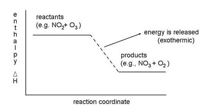
It requires additional energy and is called endothermic. If the enthalpy of the products is less than the enthalpy of the reactants, then the reaction gives off heat and is called exothermic. This relationship, stated in an equation is:

DH_reaction =SDH_products -SDH_reactants

DH_reaction < 0 , exothermic

DH_reaction > 0 , endothermic

To find out if our reaction is exothermic and possible or endothermic and (basically) not possible, look at the JPL handbook for enthalpies of common molecules. The DH values for a large number of molecules are given in the JPL document, starting on page 325.

It shows that:

DH =DH_NO3 +DH_O2 - (DH_NO2 +DH_O3)

DH = 17.6 + 0.0 - 7.9 - 34.1 = -24.4 kcal mole-1

Thus, because DH < 0, this reaction is exothermic and the reaction is possible.

Note two important thoughts:

1. The exothermicity does not determine how fast the reaction will go.
2. For reactions where H is small, that is, within a few kcal mole^-1 of 0, the change in the entropy during the reaction can determine if the reaction is possible or not.

This last effect is important in only a small number of atmospheric reactions, and we will not dwell on it. However, in reality, the enthalpy is not the determining factor, the Gibbs free energy is. The Gibbs free energy is written as:

DG =DH -DTS,

where DS is the change in the entropy, or order of the system. For DG > 0, the reaction is not energetically possible. For DG < 0, the reaction energetically can occur. For a reaction in which DH = 0, it will be energetically possible if the entropy of the products is greater than the entropy of the reactants.

Before we proceed on the question: What determines which reactions are fast and which are slow? We must consider the concept of reaction rates.

3.1.3 Kinetic theory.

Before we can talk about atmospheric photochemistry, we need to understand behavior of bulk gases, the interactions of atoms and molecules with light, and chemical kinetics. This lecture concerns the behavior of bulk gases, or kinetic theory, and some of its applications. It is useful to be familiar with the fundamental constants and atmospheric properties.

Kinetic theory provides the tools for determining a number of important properties of gases, such as the collision rate among molecules and with surfaces and transport properties such as diffusion and thermal conductivity. This lecture concerns kinetic theory and some of its useful applications.

---

Boltzmann distribution

The Boltzmann distribution of molecular properties arises from the random nature of the processes that determine those properties. We can derive the Boltzmann distribution from statistical mechanics, but instead, will simply state that the distribution of molecules over a range of energy states is given by:

n_i / n = exp(-e_i/k_BT) /ò [exp(-e/k_BT) de]

n_i / n_j = exp(-e_i/k_BT) /exp(-e_j/k_BT) = exp{-(e_i-e_j)/k_BT}

where e is the energy of the state and k_B is the Boltzmann constant k_B = R*/N_A = 1.381x10^-23 J / K.

From this expression, we can derive a number of kinetic quantities useful for atmospheric chemistry.

Mean particle speed

The mean particle speed can be determined by e = 1/2 mv² and the Bolzmann function:

f(v)dv = {(m/2pk_BT)^3/2}exp(-mv²/2k_BT) v² sin(J) d(J) d(j) dv

or, doing the integrals,

f(v)dv = {(m/2pk_BT)^3/2} exp(-mv²/2k_BT) 4pv² dv

which is the probability that a molecule has the speed between v and v+dv. We can derive the average speed, <v> = ò v f(v) dv.

average speed = <v> = [8 k_BT/pm ]^1/2 = 145.5 x [T (in K)/ M (in g/mole)]^1/2 m/s

So, the average speed of air at 273 K, where M = 29 g/mole, is about 450 m s^-1

Note that the average velocity is proportional to the square root of the temperature and the reciprocal of the square root of the mass.

The root-mean-square velocity is different from the average velocity, and is equal to:

<v²>^1/2 = [3k_BT/m]^1/2 = [3RT/M]^1/2

This expression allows us to equate particle speed to temperature:

1/2 M <v²>= 3/2 RT

Mean free path

The mean free path, l, is the average distance a molecule will travel before colliding with another molecule. The mean free path is the product of the mean time between collisions and the average velocity of the molecules. Intuitively, we would think that the important quantities would be the number density, and the "size", or cross section of the molecules (s_AB² = p(r_A +r_B)², units=cm²) and that the larger each is, the smaller the mean free path. From kinetic theory, we get that:

l= < v>/ z = 1 / [ (2)^1/2 s_ABn] = k_BT / [ (2)^1/2 s_ABp ],

where n is the number of molecules m^-3, p is the pressure in Pa, and z is the number of collisions that the molecule encounters per second.

At the surface, the mean free path is 6.6x10^-8 m. What is the vertical profile of the mean free path?

Collision frequency

The collision frequency is the reciprocal of the mean time between collisions between a molecule and all other molecules. As a result, it is equal to the mean velocity divided by the mean free path:

z = s_AB(8k_BT/ pm_AB)^1/2 n_A,

where s_AB is the average cross section of the two colliding molecules, m_AB is the reduced mass of the two molecules (1/m_AB = 1/m_A +1/m_B), and n_A is the concentrations of molecules A that the molecule B is colliding with. The units are s^-1.

Near Earth's surface, the collision frequency is 6.9x10⁹ s^-1. The collision frequency tells us something about the maximum rate that a chemical reaction can happen.

The collision rate (molecules cm^-3 s^-1) is simply the collision frequency times the concentration of molecules B.

z = s_AB(8k_BT/ pm_AB)^1/2 n_An_B

We can also associate a rate coefficient with collisions. It tells us how fast hard spheres can collide and provides a useful limit to the possible speeds of gas kinetic reactions.

k = s_AB(8k_BT/ pm_AB)^1/2

At 298 K, s_AB = p(4x10^-8)² cm²_, k_B = 1.38x10^-23 J K^-1 m_A = m_B = 0.028/6.02x10²³, the rate coefficient for collisions is about 2x10^-10 cm³ molecule^-1 s^-1. To most reactions, there are energy barriers and steric factors (orientation of molecules approaching one another) that slow the reaction rate coefficient to less that the gas kinetic rate.

Molecular flux onto a surface or through a small hole

When we start to deal with the collisions of molecules with surfaces of surfaces of such things as plants, sulfate aerosol, or raindrops, we need to know the flux of molecules (molecules cm^-2 s^-1) to that surface. We can find it using the same averaging techniques that we used to fine the mean molecular speed. In this case, we need to consider only the number of molecules traveling in one direction, say the positive x direction. After some integration, we find that:

F = ¼ n <v>.

The units are molecules cm^-2 s^-1.

The ¼ term comes from two different sources. First, of the molecules going perpendicular to the hole, only ½ on average are going towards the whole. Second, not all molecules are going perpendicular to the hole, but instead have a velocity <v>cos(θ) with respect to the hole, with the flux of molecules decreasing by cos(θ) as the angle from perpendicular increases. The average velocity and flux over all these angles results in the second ½ factor.

If we know the area of the surface, then we know the total number of molecules striking the surface.

Diffusion

The diffusion of a molecular species through air is defined by the electromagnetic interactions among molecules as they approach and leave each other (collide). The flux J of molecules (units = molecules cm^-2 s^-1) is proportional to the concentration gradient. The proportionality constant is called the diffusion coefficient, D, (units = cm² s^-1). The equation expressing this relationship is known as Fick's Law:

J = - D (dn/dx)

If we have no chemical reactions, then the total number of molecules must be conserved:

dn/dt = -dJ/dx

or

dn/dt = Dd²n/d²x

We could expand it to 3 dimensions and solve it for different cases. Instead, we consider only a result from the solutions. That is, for a release of one molecular species into air, the "characteristic" time that the molecule takes to move a distance x is given by the expression:

t = x²/2D

The diffusion coefficient is inversely dependent on the pressure, proportional to T^3/2, and inversely proportional to the square root of the particle mass. It is directly proportional to the product of the mean-free-path and the mean molecular speed.

At the surface, the diffusion coefficient is roughly equal to 0.2 cm² s^-1.

3.1.4. Reaction rate equations.

For a reaction: aA + bB ® cC + dD, where A, B, C, and D are molecules and a, b, c, and d are the number of molecules of each kind that are involved in the reaction, the rate of the reaction is given as:

R = -(1/a)d[A]/dt = -(1/b)d[B]/dt = (1/c)d[C]/dt = (1/d)d[D]/dt

From observation, it has been determined that the rate of the reaction is proportional to the concentrations (number densities) of the reactants.

Thus,

-(1/a)d[A]/dt = -(1/b)d[B]/dt = (1/c)d[C]/dt = (1/d)d[D]/dt = k[A]^a[B]^b

where k is the reaction rate coefficient

More complicated reaction sequences can be broken down into more elementary reactions. Reactions involving one molecule are called unimolecular (first order); reactions involving two molecules are called bimolecular (second order); reactions involving three molecules are called termoloecular (third order). Their rate equations are given as:

unimolecular	A ® B + C	d[A]/dt = -k^I[A]	k^I=seconds^-1
bimolecular	A + B ® C + D	d[A]/dt = -k^II[B][A]	k^II=cm^3molecule^-1s^-1
termolecular	A + B + M ® C + M	d[A]/dt = -k^III[M][B][A]	k^III=cm^6molecule^-2s^-1

M is a third body that collides but doesn't react. It is usually N₂, O₂, and H₂O. The type of M can make a difference.

A special case of bimolecular reaction is:

A + A ® B + C leads to -(1/a)d[A]/dt = -(1/b)d[B]/dt = (1/c)d[C]/dt = k[A]²

thus, d[A]/dt = -2k[A]² , but d[B]/dt = +k[A]²

These three elementary types of reactions make up all of the gas-phase reactions that occur in the atmosphere.

What are these reaction rate coefficients? They tell basically how fast the reactions will go. They are sometimes highly temperature dependent and sometimes pressure dependent. Understanding the details of reaction rate coefficients takes a great deal more time than we have here. In the next lecture, I will describe qualitatively why the reaction rate coefficient has the temperature and pressure dependencies that it does.

Lifetimes of reactants.

Very often, we need to think about the lifetime of a reactant due to reaction. We need this concept because we must think about what happens to the reactant when several processes, like gas-phase reactions, chemical destruction on a surface, and transport to other region may all be occurring simultaneously. By knowing the lifetimes for each process, we know which process controls the concentration of the reactant.

Lifetimes for different reaction types
unimolecular	1/k^I
bimolecular	1/k^II[B]
termolecular	1/k^III [M][B]
photolysis	1/J

---

3.1.5 Bimolecular reactions.

2. Why don't reactions just happen if the enthalpy of the products is less than the entropy of the reactants? What factors affect the size of the reaction rate coefficient?

To understand this question, we must look at the energy of the reactants and products. Suppose we consider a reaction in which the bond of a heteronuclear diatomic molecule is broken in a reaction with another atom and a new heterogeneous molecule is formed:

A + BC ® AB +C

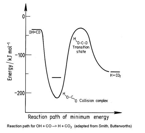
This type of reaction is called an abstraction reaction, and is very common in molecule-radical reactions, such as the reaction OH+CO ® H+CO₂. If we imagine the molecule and the atom coming close together, the electron clouds adjust, and a reaction can happen. At some distance, the three atoms may form an unstable relationship that is called an activated complex. This activated complex requires more energy than either A + BC or AB + C, but for the reaction to occur, the atoms must form it.

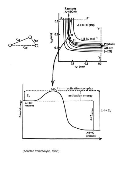
The energy required to overcome the energy barrier of the activation complex is called the activation energy, E_a.

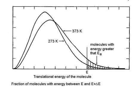
The theory that seems to capture most of the observed features of chemical reactions is called Transition State Theory. This theory assumes that once the reaction occurs, the products do not turn back into reactants; that the reactant molecules have energies distributed according the Boltzmann distribution; and that only the classical motion of the atoms and that causes the reaction are important.

Let us first consider the reason for the assumption of a Boltzmann distribution of energies of the reactant molecules. Only a small fraction of the molecules have enough kinetic energy to contribute to the energy of the activated complex, as shown in the figure below. As a result, it is only those molecules that have the higher kinetic energy that will be able to make the reaction go to products. Those with less kinetic energy will be turned back toward reactants on the reaction coordinate. Note that the higher the temperature, a greater the number of molecules that have more kinetic energy than E_a.

So we can write the reaction sequence as:

A + BC ® ABC* ® AB + C

The assumption is that the activated complex, ABC*, and the reactants, A, BC, are in equilibrium:

K* = [ABC*]/[A][BC]

This equilibrium is a quasi-equilibrium; if it were a true equilibrium, then we would not end up with accumulating reaction products. However, the assumption of equilibrium allows us to use statistical mechanics to determine the reaction rate.

This effort gives us the concentration of the activated complex. The activated complex contains extra energy and is unstable. As the molecule vibrates along the axis of the chemical bond, this vibrational energy can break the bond if

hν_B = k_BT gives ν_B = 6.1x10¹² s^-1 (Hz),

where k_B is the Boltzmann constant and T = 298 K.

The reaction rate is simply the frequency at which the bond is broken multiplied by the concentration of activation complexes, or

R = ν_B [ABC*] gives d[A]/dt = (k_BT/h)K* [A][BC]

but K* = exp(-DG*/RT) =exp(-(DH*-TDS*)/RT) = exp(DS*/R)exp(-E_a/RT)

where DH* is just the enthalpy change from the reactants to the transition state and equals E_a.

k = (k_BT/h) exp(DS*/R)exp(-E_a/RT)

where k has units of cm³ molecule^-1 s^-1. The “*” indicates a property of the activated complex.

This gives a reaction rate constant that has the form:

k = A exp(-E_a/RT)

where A is the pre-exponential term that includes issues of changes in entropy. This expression is called the Arrhenius Equation and it describes the variation of the reaction rate coefficient with temperature for bimolecular reactions, as you will see in the JPL handbook. By comparing k to the gas-kinetic collision rate, we can get some idea about how many collisions result in a reaction.

For abstraction reactions with an activation energy barrier, an increase in temperature results in an increase in the reaction rate coefficient, k.

Activation energy is not the only factor that controls the rate of a bimolecular reaction. Other factors are the orientation of the atom and molecule or molecule and molecule as they approach each other, called the steric factor. Another is the entropy change, as seen in the equation above. A third is the conservation of the quantum mechanical angular momentum, such that only certain combinations of possible quantum states of the reactant molecules may be allowed to go to products. Together, these represent the ability of the atoms in the reactants to move in a way that favors the necessary activated complex to form with the energy distributed in a way that lets the activated complex vibrate along the product side of the reaction coordinate.

Not all abstraction reactions have potential energy diagrams that are as simple as in the figure above. Consider the potential energy surface for the reaction OH + CO ® H + CO₂:

Not all bimolecular reactions have energy activation barriers. When the barrier to the reaction is low or nonexistent, then the other factors, such as the quantum mechanical effect, and the steric effect may control the reaction rate coefficient. In this case, the time that the reactants are near each other becomes important, so that accommodations can be made. Thus, these types of association reactions often have either no temperature dependence or a negative temperature dependence. That is, they go faster when the temperature is lower. An example is the reaction: HO₂ + NO ® OH + NO₂, which has an E_a/R = -250 K.

Reactions with little or no activation energy barrier, and thus zero or negative E_a/R, are usually between free radicals, as can be seen in the JPL compilation.

3.1.6 Termolecular reactions.

What about termolecular reactions? How do we determine the dependence of the termolecular reaction rate coefficient on temperature and M?

A + B + M ® C + M

Termolecular reactions usually have two molecules or atoms as reactants and one molecule as the product. M, the third body, simply carries away the excess energy. We can derive an expression for the termolecular rate coefficient by considering the following processes:

A + B ® AB* with rate coefficient k_c (combination)

AB* + M ® AB + M with rate coefficient k_s (stabilization)

AB* ® A + B with rate coefficient k_d (decomposition)

Our goal is to take these three equations and be able to write an expression for the rate equation of the form:

d[AB]/dt = k^III[M][B][A]

To do this, we write down the rate equations for each species and work to eliminate [AB*] from the expression:

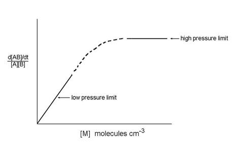
This expression has different behavior in the two limits of low and high pressure:

d[AB]/dt ={k_sk_c}/{k_s[M] + k_d}[M][B][A]

Low pressure limit:

k_s[M]<<k_d, so that d[AB]/dt = k_c[M][B][A]

High pressure limit:

k_s[M]>>k_d, so that d[AB]/dt = k_c[A][B]

The low pressure limit and the high pressure limit cover the two extreme pressure cases. What about the in between, as in the figure? It turns out that most termolecular reaction rate coefficients are in between these two extremes at atmospheric pressure.

How do we join the low-pressure reaction rate coefficient that depends on M to the high pressure limit which is independent on M? The answer is complex and beyond the scope of this class. However, the following expression has been devised and is applied to atmospheric measurements:

where k_o(T) is the low pressure rate coefficient (units: cm⁶ molecule^-2 s^-1) at temperature T, k_∞(T) is the high pressure limit (units: cm³ molecule^-1 s^-1) at temperature T, F is the form factor that defines the shape of the curve between the low pressure limit and the high pressure limit, and r_k comes from theoretical considerations. Troe derived an expression, which is used in the JPL recommendations:

Because so many atmospheric termolecular reactions are in the fall-off region between the low pressure limit and high pressure limit, it is necessary to calculate the 2^nd-order reaction rate coefficient using this expression. I suggest writing a little computer program or using an Excel spreadsheet to do the calculations whenever you need to find k.

What is the temperature dependence? To calculate the temperature dependence, JPL uses the form:

k_o(T) = k_o³⁰⁰ (T/300)^-n, where k_o³⁰⁰ and n are given and k_∞(T) = k_∞³⁰⁰ (T/300)^-m, where k_∞³⁰⁰ and m are given.

3.1.7. Chemical equilibrium.

In all reactions, there is a possibility that the products may react to form the reactants back again. In some reactions, this process is extremely unlikely, but for others, the forward and backward reactions are about equally likely. We usually apply the concept of chemical equilibrium to this later case.

For a reaction, aA + bB ↔ cC + dD, where the double arrow indicates that the reaction can go either way, chemical equilibrium states that the rate of the forward reaction equals the rate of the backward reaction.

The forward reaction has a rate coefficient k_f. The backward reaction has a rate coefficient k_r. The concentrations of A, B, C, and D adjust until the system reaches equilibrium. The equilibrium constant is defined as:

K = {[C]^c[D]^d}/{[A]^a[B]^b}

Because the rates of these two reactions must be equal at equilibrium,

K = k_f/k_r

How does the equilibrium constant change with temperature?

The equilibrium constant, K, is related to the Gibbs free energy change between the reactants and the products. The derivation of this relationship was first accomplished in the late 19th century by van't Hoff, who used the concept of chemical potential (free energy per mole of substance), to derive the expression for the change in free energy, G:

DG =DH -TDS then DG = -RT lnK and then K = exp(-DG/RT) = exp(DS/RT)exp(-DH/RT)

This expression leads directly to the van't Hoff equation:

d lnK/dT = +DH/RT²

Equilibrium constants usually have quite steep temperature dependences.

1. Complex reaction chemistry

Complex reactions are really composed on several elementary reactions - unimolecular, bimolecular, and termolecular. Even these elementary reactions can be considered to be made on individual steps, particularly the termolecular reactions, which consist of combination, stabilization, and decomposition reaction steps. However, more complex reaction chemistry consists of reactions in which atoms and molecules appear more than once as either a reactant, a product, or both.

If a reactant appears in more than one equation, then the reaction set is considered to be composed of parallel or competing reactions. For example, consider the reactions:

A + B ® products

A + C ® products

A + D ® products

All of these proceed simultaneously.

If these are all bimolecular reactions, and [A] < [B], [C], [D], then what is the lifetime of A?

If a molecule appears as a reactant in some reactions and a product in another, then the reaction set is considered to be composed of consecutive or sequential reactions.

ABC + Y ® AB + CY	Initiation reaction	(1)
AB + X ® A + XB	Propagation reaction	(2)
D + XB ® BD + X	(chain-carrying steps)	(3)
E + X + M ® EX + M	Termination reaction	(4)

In this chain reaction, (2) and (3) are considered to be the chain-carrying steps, and X is considered to be the chain carrying reactant. Usually, X is a reactive free radical (it has unpaired electrons). X and XB are intermediates.

Consider the special case where a chemical element B is shuffled between two molecules but is not consumed by a terminal reaction. That chemical B is called a catalyst and is involved in a catalytic cycle.

Consider a special case of chain reaction:

AB + X ® A + BX

BX + C ® BC + X

net: AB + C ® A + BC

X and BX are not removed in these reactions; they merely cycle one into the other. X and BX are the catalysts for converting AB + C into A + BC, and this reaction sequence is called a catalytic cycle. Catalytic cycles are very important in stratospheric chemistry in particular.

The concentration of any chemical species is the result of its chemical production, chemical loss, and transport from nearby regions that have different concentrations. This dependence can be written as the rate equation:

d[A]/dt =S_i P_i -S_i L_i [A] + S∂ ([A])/∂ x_i

where P is the production, L is the loss (NOTE: the units of L are different from the units of P), and S∂ ([A])/∂ x_i is the flux of [A] into the sampling volume. Note that the loss of A is essentially always proportional to [A].

We can define the characteristic time constant for A, or lifetime of A, as:

1/t= {1/[A]}d[A]/dt

If the chemistry is much faster than the transport, then the chemical production and loss terms will be larger in the rate equation than the transport term. Under these circumstances and in steady-state, we can ignore the transport term when solving for the evolution of [A]. Thus, the chemical lifetime can be taken as:

1/t =S_i P_i /[A] =S_i L_i implying that t = [A]/S _i P_i = 1/S_i L_i

When the production, loss, and transport of [A] balance, then d[A]/dt = 0, and the chemistry is said to be in steady-state, or if sunlight is involved, in photostationary state.

In summary, for parallel processes, the ones with the shortest lifetimes control the overall lifetime. For sequential processes, the ones with the longest lifetimes control the overall lifetime.

3.5 Heterogeneous chemistry and aqueous-phase chemistry

3.5.1 Heterogenous processes

Heterogeneous processes are a combination of chemistry and transport within different phases and across the phase boundaries. All of these processes must be taken into account because, depending on the atmospheric constituents and environmental conditions, different processes can be the slowest, thus controlling the overall rate of the heterogeneous chemistry.

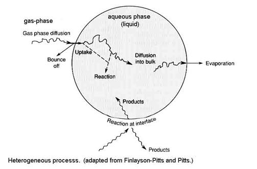
Four main processes are responsible for the distribution of an atmospheric constituent between the gas-phase and aqueous phase:

1. gas-phase transport to the surface, designated by Γ_g

2. uptake at the surface (called interfacial exchange), designated by a

3. aqueous-phase transport, designated by Γ_sol

4. chemical reaction in solution, designated by Γ_rxn

If the solid phase is involved, such as on ice, then steps 3 and 4 are replaced with chemical reaction on the surface. Heterogeneous processes involving the solid phase is similar to heterogeneous processes in the liquid phase, so we will do the liquid phase first.

The designations for all processes are made into unitless probabilities in a way that the different processes can be compared. We are asking: What is the chance that each process will happen to a gas molecule at each step?

The net uptake probability, g_net, is simply the probability that a gas molecule will be taken up by the liquid drop. Note that gas-phase diffusion, uptake at the surface and processes that are occurring inside the drop are all in parallel, while aqueous-phase transport and chemical reaction in solution occur in series. As a result, the net uptake is given by the other terms as the expression:

where G_g is the gas conductance, a is the mass accommodation coefficient, G_sol is liquid-phase conductance, and G_rxn is the rate of reaction in the liquid normalized by the collision rate of molecules with the drop surface. All of these terms are unitless.

Let’s look at each one of these terms in more detail to see the most important terms in different conditions.

1. The convection-diffusion equation is given by the expression:

where n_g is the concentration of the trace gas, D_g is the gas-phase diffusion coefficient (~0.2 cm² s^-1), F_g is the flux of the gas, with the first term being advection and the second term being diffusion. The solution is complicated and depends on the assumptions. In steady-state, ¶n_g/¶t = 0 and u = 0. The equation for a spherical particle of radius a and diameter 2a=d becomes:

The time constant for establishing this steady-state is given by the expression:

For d ~ 10 mm, t_dg ~ ms; for d ~ 1 mm, t_dg ~ 0.01 s. Thus, we see that gas-phase transport to a small drop, like a cloud drop or an aerosol, is slow, while gas-phase transport to a large particle, like a raindrop, is fast.

The flux of molecules to the surface is:

where n_gsfc is assumed to be 0. The total number of molecules diffusing to the surface is the flux times the surfaced area:

F_g 4πa² = 4πD_g a n_g.

Recall that the number of collisions of gas molecules per unit area of surface is:

The gas conductance is the ratio of the diffusion flux to the collision rate, G_g = 8D_g/<v>d

When the particle is large enough that the gas can be treated as a continuum, K_n = λ/a << 1, where λ~7x10^-8 m,

Since D_g ~ 0.2 cm² s^-1, <v> ~ 4x10⁴ cm s^-1, if d = 10 mm = 10^-4 cm, G_g ~ 0.5; if d = 1 mm, G_g ~ 4x10^-4. We will be comparing these values to those of the other processes.

2. Interfacial exchange.

When molecules collide with a surface, they can either stick and become incorporated or they can bounce off. The mass accommodation coefficient, or sticking coefficient, a, is given by the expression:

a = incorporation flux / impingement flux

a must be measured in the laboratory. Generally, 10^-6 < a < 1.0. You can view the values for a in the JPL book.

3. Solubility and diffusion in the liquid phase (Γ_sol).

The concentration of the chemical in the liquid phase can be represented by n_l, and has units of molecules cm^-3. It’s flux across a surface in the liquid is given by the expression:

The rate of transfer of molecules across this surface inside the liquid is just the liquid diffusion coefficient, D_l, times the gradient of the chemical concentration at an internal surface:

where R_t has units of molecules cm^-2 s^-1, D_l (typically ~2x10^-5 cm² s^-1), n_l,interface is the chemical concentration at the interface between the liquid and the air, and n_l,bulk is the chemical concentration in the bulk of the liquid, and t is the time from first exposure of the drop to the chemical.

When there is no chemical in the bulk phase, then the rate of transfer is highest:

where τ_l is the characteristic time, d is the diameter. For 10 mm diameter drops, τ_l ~ 10^-3 s.

However, note that as time goes on, the concentration in the bulk approaches the concentration at the interface. Eventually, an equlibirum is reached and mass transfer ceases. However, uptake by the liquid is not a one-way process. Evaporation (or desorption) can also occur. For a chemical species A, the incorporation flux depends on n_A, or for a given temperature, the partial pressure of A, p_A. On the other hand, the desorption flux depends on the amount of A in the aqueous phase, n_{l,interface,A} = [A(aq)]. At equilibrium, the incorporation flux and the desorption flux become equal. Thus, p_A becomes a measure of [A(aq)]. The coefficient of proportionality is called the Henry’s Law Coefficient, H, which we will talk about much more in the next lecture.

The concentration at the interface, n_l,interface, can be replaced with the related gas-phase concentration or partial pressure:

p_A = n_gk_BT/p_o in units of atm, since p_o is 1 atm. Thus, n_{l,interface,A} = H n_g k_BT/p_o, and

Where, as in the case of the gas-phase transport, Γ_sol is the ratio of liquid-phase transport divided by the flux of molecules to the surface. As t ® ∞, Γ_sol ® 0.

4. Liquid-phase reaction.

The rate equation is given by the expression:

where D_l is the liquid-phase diffusion coefficient, n_l is the chemical concentration in the liquid phase, and k is the irreversible, first-order liquid-phase reaction rate coefficient (s^-1). We can solve this equation for the case where n_l is initially 0 in the bulk phase at time t=0 and that the concentration in the thin interfacial layer is in equilibrium between the gas and liquid phases, according to Henry’s Law. For kt >>1 (i.e., either a very fast reaction or a reaction in which the reaction product’s solubility is large), the rate of transfer of molecules by reaction in the liquid phase becomes the expression:

Combining all of these terms, we can write down an expression for the net uptake coefficient:

We have several limiting cases to consider (Finlayson-Pitts and Pitts).

1. Fast gas transport, high solubility, and / or fast reaction.

g_net ~ a. The mass accommodation coefficient determines the net uptake. This case occurs with some gases for stratospheric aerosols.

2. Fast gas transport, low solubility and / or fast reaction.

Γ_sol << Γ_rxn.

3. High solubility (and / or short exposure times), no reaction.

4. Gas transport and mass accommodation fast, solubility low, and slow reaction.

5. Low solubility and no reaction.

A way to compare the importance of the four steps in heterogeneous processes is to consider the characteristic times for each process. Remember that the faster of liquid-phase transport or liquid-phase reaction will dominate the in-liquid process, while the slowest precess of gas-phase transport, mass accommodation, or the faster of liquid-phase transport or liquid-phase reaction determines the overall net uptake.

Characteristic times for the four processes involved in net uptake
heterogeneous process	expression for characteristic time (s)
gas-phase diffusion
mass accommodation
liquid-phase diffusion
liquid-phase reaction

Remember that “a” is the particle radius.

Equilibrium conditions.

In many cases, equilibrium is rapidly established between the uptake and the desorption of a chemical between the gas and liquid phases. Even when reactions are occurring in the liquid-phase, a quasi-equilibrium exists between the gas and liquid phases. This greatly simplifies the calculations for aqueous phase oxidation.

Recall that the molecular flux to a surface is given by the expression: F = 1/4 n_A <v_A> where

n_A = p_A/k_BT and <v_A> = (8k_BT/pm_A)^1/2

Both absorption and desorption are constantly occurring. The absorption depends on the concentration of A, or the partial pressure of A and the desorption depends on the concentration of A in the solution. Equilibrium is rapidly established between the absorption and the desorption. Thus,

F_A^des(T,[A(aq)]) = a_AF_A = (a_Ap_A^sat)/(2pm_Ak_BT)^1/2

This equilibrium condition defines p_A^sat. The larger p_A^sat, the greater the desorption flux.

Thus by definition,

in the gas, [A(g)] is defined as n_A = p_A/k_BT <==> p_A = [A(g)] k_BT

in the liquid, the mole fraction is defined as c_A = [A(aq)]/{[H₂O] + [A(aq)]}

The molar concentration of water, [H₂O], is 55.5 mole L^{-1 =} 55.5 M (molar).

Combining these definitions with the concept of equilibrium between absorption and desorption fluxes, we arrive at the concept that p_A^sat is proportional to c_A. Solutions that obey this proportionality obey Raoult's Law.

When c_A = 1, p_A^sat = p_A^o, the vapor pressure of a pure solution.

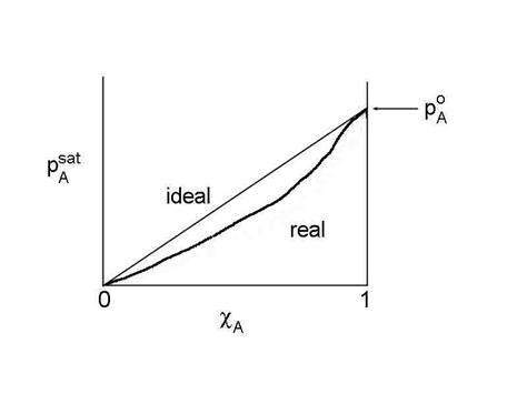
Unfortunately, most solutions are not ideal across the range of 0 < c_A< 1. However, we can still use the concept of Raoult's Law by forcing the relationship to hold. We define a new measure of the liquid concentration, called the activity, a_A, where:

p_A^sat /p_A^o = a_A = g_A c_A

where g_A is called the activity coefficient, which is a function of c_A, and p^o_A is the saturation vapor pressure when c_A=1. This is NOT the same as the gamma that we used for the net uptake. Don’t get them confused. This equation is the generalized form of Raoult's Law.

When the solution is ideal, g_A=1. For non-ideal solutions, g_A may be either less than or greater than 1. If g_A< 1, then A is more soluble than ideal; if g_A> 1, then A is less soluble than ideal. Raoult's Law tends to stay valid for solvent (component with c approaching 1).

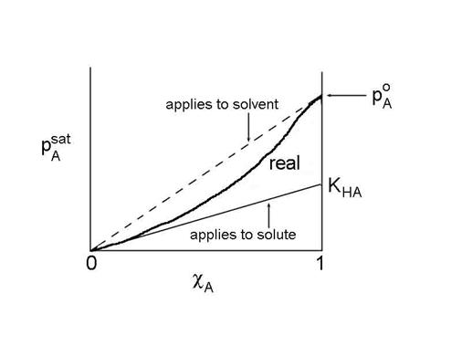
The solute also obeys a linear relationship, called Henry's Law:

p_A^sat = K_HA c_A

where K_HA = g_A,0 p_A^o. We can move the coefficient over to the pressure side of the equation to get the more familiar form of Henry's Law:

c_A = H_Ap_A

where H_A is defined as H_A = 1/ K_HA

This is true as long as the solvent molecules interact mostly with solvent molecules. However, the reference state is not a pure liquid (p_A^o), but rather, the reference state is a hypothetical state based on a linear extrapolation from infinite dilution (c_A goes to 0).

• Extrapolate to the dilute solution limit to find K_HA.
• The solute obeys Henry's Law.
• The solvent obeys Raoult's Law.

Temperature dependences of the Henry’s Law Coefficients.

Just as for gas-phase equilibria, the temperature dependence of the Henry’s Law Coefficients obeys the van’t Hoff equation:

Assuming that DH_A is constant and integrating this expression over small temperature ranges, we get the expression:

Different chemicals exhibit a wide range of Henry’s Law Coefficients, as can be seen in the attached table.